Examples

Example 1: A simple network of coupled Montbrio model nodes.

Starting with a few imports

../examples/00_intro.py

import os
import vbjax as vb
import jax.numpy as np
os.makedirs('images', exist_ok=True)

This example shows how to use the vbjax library to simulate a network of Montbrio model nodes. The network is defined by the function network which takes as arguments the state of the network and the parameters of the model. The function returns the time derivative of the state of the network.

def network(x, p):
    c = 0.03*x.sum(axis=1)
    return vb.mpr_dfun(x, c, p)

The function make_sde is used to create a function loop that simulates the network for a given time interval and a given set of initial conditions.

_, loop = vb.make_sde(dt=0.01, dfun=network, gfun=0.1)

The function vb.randn is used to generate a set of noise samples. The dimesions are (time, state, node). The first noise sample is used as the initial condition of the network. The remaining noise samples are used to generate the noise term of the stochastic differential equation.

zs = vb.randn(500, 2, 32)

The function loop takes as arguments the initial conditions of the network, vector of noise samples, and the parameters of the model. The function returns the state of the network at each time step.

xs = loop(zs[0], zs[1:], vb.mpr_default_theta)

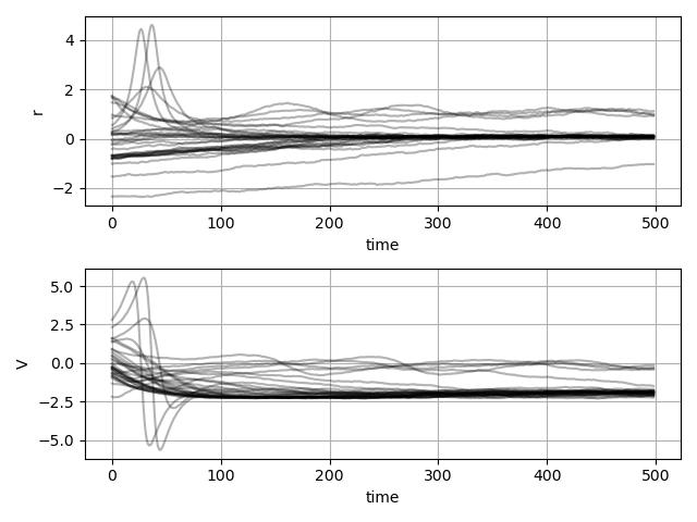
The function vb.plot_states is used to plot the state of the network. The function takes as arguments the state of the network, the format of the plot, and the name of the output file.

vb.plot_states(xs, 'rV', jpg='images/example1', show=False)

Example 2: Consider a network of coupled Montbrio model nodes and sweep over the parameters of the model.

Starting with a few imports

../examples/01_sweep.py

import os
import time
import vbjax as vb
import pylab as pl  
import jax, jax.numpy as np
os.makedirs('images', exist_ok=True)

This example shows how to use the vbjax library to simulate a network of Montbrio model nodes. The network is defined by the function network which takes as arguments the state of the network and the parameters of the model.

def network(x, p):
    r, v = x
    k, _, mpr_p = p
    c = k*r.sum(), k*v.sum()
    return vb.mpr_dfun(x, c, mpr_p)

The function noise is used to generate the noise term of the stochastic

def noise(_, p):
    _, sigma, _ = p
    return sigma

The function run is used to simulate the network for a given set of parameters.

def run(pars, mpr_p=vb.mpr_default_theta):
    k, sig, eta = pars                      # explored pars
    p = k, sig, mpr_p._replace(eta=eta)     # set mpr
    xs = loop(rv0, zs, p)                   # run sim
    std = xs[400:, 0].std()                 # eval metric
    return std                              # done

Then prepare the simulation

n_nodes = 8

define the number of nodes in the network.

using_cpu = jax.local_devices()[0].platform == 'cpu'
if using_cpu:
    run_batches = jax.pmap(jax.vmap(run, in_axes=1), in_axes=0)
else:
    run_batches = jax.vmap(run, in_axes=1)

defines the engine to be used for the simulation. If the simulation is run on the CPU, then the simulation is parallelized over the cores of the CPU using jax.pmap. Otherwise, the simulation is parallelized over the GPU using jax.vmap.

then we prepare the network and the noise samples

# prepare network
_, loop = vb.make_sde(0.01, network, noise)
rv0 = vb.randn(2, n_nodes)

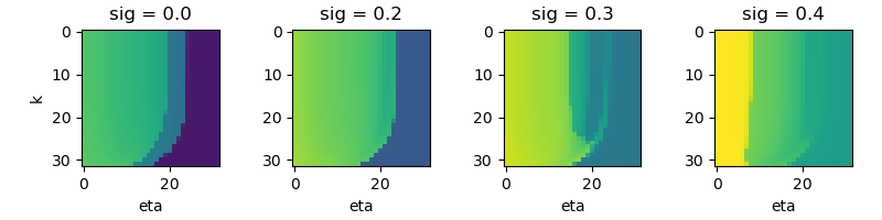
The rest run the simulation on set of parameters and plot the results.

# sweep sigma but just a few values are enough
sigmas = [0.0, 0.2, 0.3, 0.4]
results = []
ng = vb.cores*4 if using_cpu else 32

for i, sig_i in enumerate(sigmas):
    # create grid of k (on logarithmic scale) and eta
    log_ks, etas = np.mgrid[-9.0:-2.0:1j*ng, -4.0:-6.0:1j*ng]

    # reshape grid to big batch of values
    pars = np.c_[
        np.exp(log_ks.ravel()),
        np.ones(log_ks.size)*sig_i,
        etas.ravel()].T.copy()

    # cpu w/ pmap expects a chunk for each core
    if using_cpu:
        pars = pars.reshape((3, vb.cores, -1)).transpose((1, 0, 2))

    # now run
    result = run_batches(pars).block_until_ready()
    results.append(result)

toc = time.time()
print(f'elapsed time for sweep {toc - tic:0.1f} s')


pl.figure(figsize=(8, 2))
pl.figure(figsize=(8,2))
for i, (sig_i, result) in enumerate(zip(sigmas, results)):
    pl.subplot(1, 4, i + 1)
    pl.imshow(result.reshape(log_ks.shape), vmin=0.2, vmax=0.7)